I was reading this post by Su Jianlin when one sentence stopped me:
Besides the KV cache, decoding now has another variable — MTP, or speculative decoding, whose idea is to trade compute for speed. But MLA behaves during decoding like an MQA with head_dims=512+, and has already consumed most of the compute up front, so “MLA+MTP” tends to lose out.
My first reaction was: what does that mean? Why would MLA “consume compute up front” during decode? And why should it conflict with MTP that its decode FLOPs come out equivalent to a head-dim-512+ MHA?
Following the question down led to something classic, but unusually pretty when applied to attention: arithmetic intensity — FLOPs per byte moved.
And the answer turns out to be surprisingly clean (everything below assumes a BF16 KV cache):
- Reduce MHA all the way down and its AI comes out to exactly 1;
- GQA and MQA are just as clean — they depend on nothing but head counts. Context length and head dim cancel out completely;
- MLA has the same shape again, independent of the latent dim too, just with a constant of a little under 2 in front.
Lined up, here is the AI of the attention core for a single-token decode:
| Attention | what the cache holds | AI, roughly |
|---|---|---|
| MHA | each query head has its own K and V | 1 |
| GQA | a group of query heads shares one K and V | query heads / KV heads |
| MQA | all query heads share one K and V | number of query heads |
| MLA | one latent, K and V both expand from it | ~2 × number of query heads |
Sections 2 and 4 derive those four rows. The first three are the same formula with different KV head counts; the constant on the last row comes from somewhere else entirely.
And that constant of a little under 2 is just enough to move attention decode on many current GPUs from clearly memory-bound to sitting near the roofline knee. Stack MTP on top and the workload tips over into compute-bound — which is exactly why Su says MLA is unfriendly to MTP.
This post works through the whole derivation.
This one is written out in detail — starting from how you count FLOPs in a matmul, with every matrix shape spelled out. If you already know the structure of attention and what decode computes, section 2 can be skimmed down to the result in 2.5, then jump to section 3.
1. What arithmetic intensity is
The definition is simple:
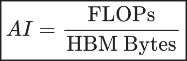
That is: for every byte pulled in from HBM, how many floating-point operations do you get out of it.
Low AI means the GPU spends most of its time moving data. High AI means each piece of data gets reused for a lot of arithmetic once it arrives.
The hardware has a matching threshold:

In the idealized roofline model:

and

Using dense BF16 tensor-core throughput, the theoretical balance points of a few common cards:
| GPU | Dense BF16 Peak | HBM Bandwidth | Theoretical Balance Point |
|---|---|---|---|
| H100 SXM | ~989.5 TFLOP/s | 3.35 TB/s | ~295 FLOP/B |
| H200 SXM | ~989.5 TFLOP/s | 4.8 TB/s | ~206 FLOP/B |
| B200 (HGX) | ~2.25 PFLOP/s | ~8 TB/s | ~281 FLOP/B |
Sources: NVIDIA H100, NVIDIA H200, NVIDIA HGX B200, NVIDIA DGX B200.
No real kernel saturates peak FLOPs and peak bandwidth simultaneously, so treat these as a roofline upper bound for building intuition rather than a line you would see in a profiler. “A few hundred FLOP/B” is the magnitude to remember; it gets compared against later.
One caveat worth stating up front: AI is a ratio. It answers “which side of the roofline are you on”, not “which approach is faster.” Numerator and denominator can both grow and leave AI untouched while everything gets slower. Section 5 has a concrete case: two algorithms computing the same thing, where the one with the higher AI does 120× the FLOPs.
What follows only counts the KV-related part of attention:
For one decoded token: from its hidden state, compute Q, K and V, read in the KV cache, and carry through to this layer’s attention output.
Softmax is small next to the two big matmuls and is left out. The goal is not to estimate whole-layer latency; it is to isolate one question: what does changing the attention structure do to the arithmetic intensity of that stretch?
Sections 2 through 4 handle decode only (one token at a time, history read from cache). Prefill — computing an entire sequence at once — waits until section 5, where it turns out the same model wants the opposite algorithm in the two phases.
PS: why not count the final WO too? Because it has nothing to do with which attention structure you picked. WO always receives the concatenated per-head outputs, whose width depends only on Hq and dv — how the KV side is organized is invisible to it, and MHA, GQA, MQA and MLA all hand it something the same width. Like the Q/K/V projections it is a weight-times-vector: it never touches the KV cache, does not grow with L, and at batch = 1 its AI is fixed at 2/b. Including it adds the same constant to every structure and dilutes the comparison. Same for the MLP and for communication.
2. One formula for MHA / GQA / MQA
2.1 How to count FLOPs
An (m × k) matrix times a (k × n) matrix takes m·n·k multiply-accumulates (MACs). One MAC is a multiply plus an add, so 2 FLOPs:

2.2 MHA, briefly
The most basic attention is MHA: split the hidden state into heads, let each head compute its own Query, Key and Value, run attention independently, then concatenate.
Start with the shapes. The layer receives the current token’s hidden state:

Three projections turn it into Query, Key and Value. In MHA all three have the same head count, but GQA and MQA later reduce the K/V head count, so it gets its own symbol: Hq query heads, Hkv KV heads, with MHA being the case Hkv = Hq.
One thing to settle here: the Key head count and the Value head count are not required by the math to match — 8 groups of K and 4 of V would work fine on paper. But no real model is built that way: K and V are cached in pairs, and storing a position’s k always means storing its v. This post follows that convention and calls both Hkv.
As for head dims: Query and Key must match, or q and k cannot be dotted — call it dk. The Value dimension may differ; call it dv.

Per head:

The new k and v are appended to the KV cache. With history length L, the layer’s cache is:

Then each query head does three steps. Write g(h) for the KV head that query head h uses (in MHA, g(h) = h):
One — score. Dot the current query against all L cached keys, a (1 × dk) by (dk × L) product:

Two — normalise. Softmax turns scores into weights; the shape does not change:

Three — weighted sum. Multiply the weights into Value, a (1 × L) by (L × dv) product:

The Hq per-head outputs concatenate into the layer’s attention output.
2.3 FLOPs
Three parts, each with shapes substituted into 2mnk.
One — compute this token’s Q, K, V. Three (1 × dmodel) by (dmodel × ·) products, so m = 1:

Two — score. Per query head, one (1 × dk) by (dk × L) product, times Hq heads:

Three — weighted sum. Per query head, one (1 × L) by (L × dv) product:

All three together are the layer’s attention arithmetic:

The two terms behave completely differently: Fproj is independent of history length L, since it only handles the current token, while the second term is proportional to L, because it sweeps the whole history. Their ratio, to an order of magnitude:
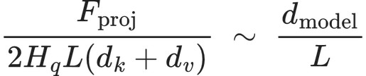
(Substituting MHA’s Hkv = Hq and dk = dv gives exactly 1.5 dmodel/L.)
That ratio is not as small as it sounds. With dmodel = 7168 it is 10752/L: at L = 8K the projections cost more than attention (1.3×), at 32K they are 33%, and it takes over a hundred thousand tokens to drop below 10%.
So dropping Fproj is not justified by its being small. What justifies it is that it is irrelevant to the comparison — Fproj is a weight-times-vector, reading weights rather than the KV cache, with AI fixed at 2/b whichever attention structure you choose. Fattn is the only term that grows with L and the only one the structure changes. The AI below keeps just that:

That said, do not forget the Fproj path itself. Section 3 shows that what MLA does is precisely to move work that would have been multiplied by L back onto that L-independent path.
2.4 HBM bytes
Let each element take b bytes; BF16 means b = 2.
The cache holds Hkv keys and Hkv values, each position’s key dk wide and value dv wide, across L positions:

This assumes a fused attention that does not write the L-length score/probability matrix back to HBM.
The three projection weights are read from HBM too, of course. But they are weights rather than KV cache, and at batch = 1 a matrix-times-vector has AI fixed at 2/b regardless of attention structure, so they do not affect the comparison between structures below.
2.5 Divide
Keeping only the part that grows with L:
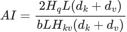
L cancels, and (dk + dv) cancels as a block:
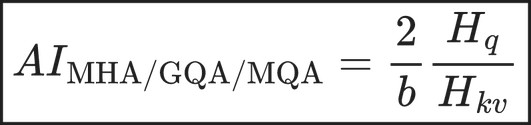
With BF16, b = 2:
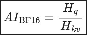
Here is the pretty part: context length L and both head dims cancel out entirely.
One quantity is left:
2.6 Three special cases
MHA, GQA and MQA differ only in what Hkv is:
| structure | Hkv | meaning | BF16 AI |
|---|---|---|---|
| MHA | Hkv = Hq | one KV per query head | 1 |
| GQA | 1 < Hkv < Hq | shared within a group | Hq / Hkv |
| MQA | Hkv = 1 | shared by all | Hq |
So MHA → GQA → MQA is one formula with Hkv sliding: FLOPs do not drop when KV heads are removed, but the history read from HBM does, because one KV is reused by more query heads.
That is the first layer of data reuse.
2.7 Real models
For example:
- Qwen2.5-7B: Hq = 28, Hkv = 4;
- Mixtral-8x7B: Hq = 32, Hkv = 8;
- Falcon-7B: 71 query heads with
multi_query=true, i.e. true MQA.
So for BF16 single-token decode, the AI of this part is roughly:
| Model | Attention | Hq | Hkv | BF16 AI |
|---|---|---|---|---|
| Qwen2.5-7B | GQA | 28 | 4 | 7 FLOP/B |
| Mixtral-8x7B | GQA | 32 | 8 | 4 FLOP/B |
| Falcon-7B | MQA | 71 | 1 | 71 FLOP/B |
At this point MQA has taken cross-head KV reuse as far as it goes: every query head shares one K and one V, and AI equals the query head count.
Which is also where it gets stuck: MQA’s AI ceiling is the query head count, and that number does not grow. Common models have 32, 64 or 128 query heads; Falcon-7B’s 71 is already on the high side, and the count is fixed by the architecture — you cannot simply add heads to buy AI. Against the few-hundred FLOP/B balance points from section 1, piling on query heads alone cannot get there.
And note the last few words:
one K, and one V.
K and V are still two separate pieces of data.
That is what MLA changes next.
2.8 What about prefill?
Everything above was decode. What do the same formulas give for prefill?
Prefill computes the whole input at once. Let the input length be L (the same symbol as above — in decode it is the history, in prefill it is the input length itself). Every token attends to all tokens before it, so each K and V gets used by roughly L query tokens — the reuse is free. Dividing the same way:
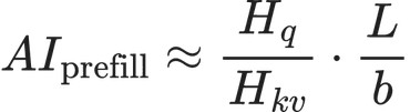
That is the decode AI multiplied by L/b. Against H100’s 295 FLOP/B:
| decode AI | L needed to pass 295 in prefill | |
|---|---|---|
| MHA (Hq = Hkv) | 1 | 590 |
| GQA (32 / 8) | 4 | 148 |
| MQA (32 / 1) | 32 | 18 |
In prefill even plain MHA is compute-bound — past six hundred or so tokens it is over the line, and GQA/MQA cross within a few dozen. There is no memory-bound problem to discuss in prefill at all.
Worth noting too: GQA and MQA do not change prefill FLOPs whatsoever, because FLOPs depend on Hq and not Hkv. They only push an already-over-the-line AI higher, and shrink the cache.
So:
The whole MHA → GQA → MQA → MLA line is a decode story. Reuse in prefill is free and there is nothing to fix; these structures exist because decode has exactly one query token and therefore no reuse at all.
3. MLA’s latent cache
Editor’s note: to keep the core structure clear, the next few sections ignore RoPE. It does not change the conclusion; putting it back is covered in appendix A at the end.
What MLA changes is not attention’s final form:

but the parameterization of the cached K and V.
For history token j, the hidden state is first compressed into a KV latent shared by all heads. The D stands for down-projection: WDKV is the matrix that takes the dmodel-wide hidden state down to a much narrower dc:
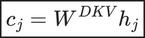
Two different h’s here, so watch the subscripts. The h in hj is the hidden state and j indexes the token: it is history token j’s vector at this layer, on its way into attention. The h in qh and WhK below is the head index. Throughout this post, head indices ride on the operators and token indices ride on the vectors.
where:
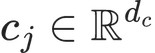
Head h’s K and V both expand out of that one latent:
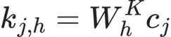
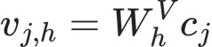
So what used to be cached,
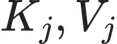
now only needs to be:

Put Kimi K3’s numbers in: 96 heads, K and V head dims both 128, so one KV is 128 + 128 = 256 numbers. How much you store per token per layer is then just how many copies you keep:
| structure | numbers per token per layer | if all 93 layers used this structure (32K context, BF16) |
|---|---|---|
| MHA (96 KV) | 256 × 96 | 139.5 GB |
| GQA (8 KV) | 256 × 8 | 11.6 GB |
| MQA (1 KV) | 256 × 1 | 1.45 GB |
| MLA (one latent) | 512 | 2.91 GB |
48× smaller than MHA and 4× smaller than 8-group GQA — but twice as large as MQA.
That last column is a hypothetical, and K3 is not actually shaped like it, for two reasons. Layer count: only 24 of K3’s 93 layers are full attention (
full_attn_layersin the config); the other 69 are KDA, which carries a recurrent state that does not grow with token count and cannot be added to a per-token KV cache. Width: the table follows this section’s convention of ignoring RoPE, while K3 actually stores 512 + 64 = 576 numbers per token (appendix A.2 covers those 64). Put both back and K3’s real KV cache at 32K in BF16 is 24 × 576, about 0.84 GB.
So MLA’s selling point was never “smallest cache”; on cache size alone it loses to MQA. What it buys is something else: that one latent plays the role of both K and V, whereas MQA’s 256 is 128 of K and 128 of V doing separate jobs. Section 4 prices what that is worth.
But it immediately raises a problem: if every generated token re-expands all L cached latents through WK and WV, you have traded an HBM problem for an enormous compute one.
The clever part of MLA at decode is matrix absorption / reassociation.
3.1 K-side absorption
The original content score:
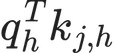
Substituting:
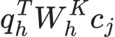
By associativity of matrix multiplication this can be rewritten:

Which means there is no need to generate K for each of the L cached latents.
Instead, transform the single current query token once, pulling it into latent space — the resulting q̃h can be read as “the query, in latent space”:

then dot it against the whole history directly in latent space:

The direction is reversed: instead of expanding every cached latent into a K and comparing the query against it, the query is moved into latent space once and compared against the latents as stored. The scores are identical, but the second way never touches the history.
3.2 V-side absorption
Likewise, the original attention output:
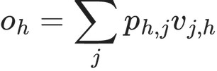
Substituting vj,h = WhVcj:
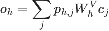
Pulling the constant matrix outside the sum:
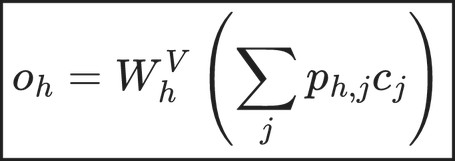
So PV can also happen entirely in latent space:

with a single WhV projection applied to the one latent output at the end.
3.3 Why the projection did not get expensive
This is the part I misread at first.
Without absorption, every generated token has to re-expand every cached cj — computing kj,h = WhKcj and vj,h = WhVcj for each head. The longer the history, the more times you do it, so the cost carries a factor of L:
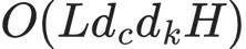
After absorption, the extra K-side and V-side projections only touch the current query or the final output:

They are no longer multiplied by context length L.
The part that grows with history becomes:
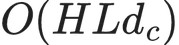
So at long context, those few projections on the current token shrink steadily relative to reading the whole history.
Put another way:
MLA does not make the projection disappear. It changes the order of association, moving an expensive projection off the sequence’s O(L) dimension and leaving it on the O(1) current-token path of each decode step.
Same result, very different compute graph.
3.4 So why not just cache the hidden state
All of this invites an obvious follow-up. Plain MHA’s kj,h and vj,h are themselves linear projections of the same hj, so why not cache hj directly? That drops WDKV entirely and looks like MLA minus one down-projection.
The algebra does work. Swap cj for hj in section 3.1’s step and the associativity still holds:

The V side is section 3.2 verbatim:

So (still ignoring RoPE) ordinary attention can cache hj alone and absorb WK and WV into the two sides, never materializing the cached K and V. Seen that way it is just MLA with cj = hj and WDKV = I.
The math is fine. The trouble is two bills. Below, let dk = dv = dh and dmodel = Hqdh, which is how most dense models are built — Qwen3-8B’s 32 × 128 = 4096, for instance.
Bill one: storage. The hidden state is dmodel numbers per token per layer and the KV is Hkv(dk + dv). Divide, and dh cancels:
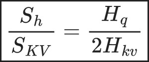
Two head counts, nothing else. Which sends the three structures in different directions:
- MHA (Hkv = Hq): ratio 1/2, caching hidden halves the cache;
- GQA (Hkv < Hq): depends on Hq / Hkv, and may well not help;
- MQA (Hkv = 1): ratio Hq/2, which at 32 query heads is 16×.
Put Qwen3-8B in (dmodel = 4096, Hq = 32, Hkv = 8, dh = 128), per token per layer in BF16:
| what you cache | per token per layer | BF16 |
|---|---|---|
| hidden (one 4096-wide vector) | 4096 numbers | 8 KiB |
| GQA KV (8 × 128+128) | 2048 numbers | 4 KiB |
Caching one hidden state is twice the size of storing eight K/V pairs. A single 4096-wide vector is simply wider than 8 × 256 = 2048 — GQA cuts the number of copies, and the hidden state is one indivisible copy.
Bill two: compute. Once absorption moves WhK to the query side, scoring is no longer dh against dh; it is a dot product over the width of whatever you cached. So the reduction width per (query head, cached token) pair goes from dk + dv = 2dh to 2dmodel:
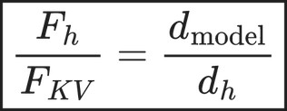
Given dmodel = Hqdh, that ratio is just Hq. For Qwen3-8B it is 4096 / 128 = 32×. At L = 4096, one layer’s attention core: 4 × 32 × 4096 × 128 ≈ 67.1 MFLOPs for ordinary GQA, 4 × 32 × 4096 × 4096 ≈ 2.15 GFLOPs for cached hidden.
Note what is absent from that ratio: Hkv. Whether GQA cuts to 8 KV copies or MQA cuts to 1, this bill does not move a cent — cutting copies changes storage, not this width.
Put the two bills together and the shape of the answer is unexpectedly tidy: caching the hidden state always costs Hq× the attention core, whether you run MHA, GQA or MQA. The only column where the three differ is storage, and only MHA’s entry there is positive.
- MHA: save 2× on cache, pay Hq× on the attention core. Tens of times for a factor of two is a bad trade.
- GQA / MQA: the number of KV copies has already been cut once, so the hidden state is usually the larger of the two — both bills go up, and there is nothing left to trade.
Which is where MLA sits. MLA neither takes WDKV to be the identity (that is caching hidden) nor stores the expanded per-head K and V; it learns an intermediate width dc:

All three side by side (reduction width is per query head per cached token, summing the QK and PV contractions):
| what you cache | width per token per layer | reduction width | K3’s numbers |
|---|---|---|---|
| expanded per-head K/V | 2Hkvdh | 2dh | 256 |
| KV latent (MLA) | dc | 2dc | 1024 |
| full hidden state | dmodel | 2dmodel | 14336 |
In the reduction-width column, MLA’s 1024 sits squarely between 256 and 14336. So MLA does take a middle point between storage and compute, and the part that matters is that the middle point is learned. WDKV is a trainable low-rank bottleneck with two jobs at once: narrow enough to pay off in HBM, yet informative enough that each head can still recover its own K and V. The identity map does the second and not the first; simply cutting the width does the first and not the second.
So MLA’s key idea is not that it caches an intermediate representation — ordinary attention can do that too. It is that it learns a representation far narrower than the hidden state which still reconstructs every head’s K and V, buying a large cut in HBM traffic with a bounded increase in compute.
Pricing that increase is exactly what sections 4 and 5 do.
Thanks to Nan Jiang (@nanjiangwill) for this angle — coming at MLA from “why not just cache hidden” makes it much clearer than calling it KV compression does.
4. Why MLA’s AI doubles
Per section 3, each cached token stores one latent.
In MLA all query heads share that latent, so there is no “KV head count” dimension left; a single head count suffices, denoted H, which is the earlier Hq.
Per cached token:
4.1 FLOPs
One — the parts independent of history length. This one new token has to: compress its hidden state into a latent (2dmodeldc), compute its own query (2dmodelHdk), fold WK into that query (the absorption of 3.1, 2Hdkdc), and project the latent output back per head (2Hdcdv). All of it applies to the current token only; call it Ffixed.
Two — the parts that sweep the history. After absorption both the scoring and the weighted sum run on the latent, width dc:

Together:

For DeepSeek-V3 (dmodel = 7168, H = 128, dc = 512, dk = dv = 128), Ffixed ≈ 276 MFLOP versus 0.26 MFLOP × L — a ratio of about 1052/L, so 13% at L = 8K and 3% at 32K.
Dropping Ffixed is justified as before: it does not vary with L and does not participate in what is being compared. Keeping only the part that grows with L:

4.2 HBM bytes
Here is the crux.
The history no longer has separate K and V caches, only one:
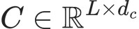
so under a fused kernel:
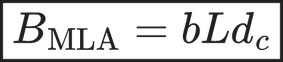
Note there is no factor of 2 for K plus V in the denominator.
Once that latent is read from HBM it:
- takes part in QK;
- takes part in PV.
So:
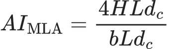
giving:
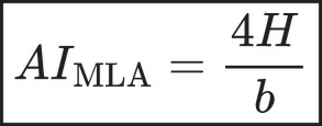
With BF16, b = 2:

As in 2.5, the latent dim dc cancels here too: the AI has nothing to do with how wide the latent is, only with the head count. Widening the latent rank from 512 to 1024 doubles the KV cache and leaves this AI untouched.
The whole MLA AI story in one paragraph:
MQA already had every query head share the KV, reaching AI = H. MLA goes further and compresses what used to be two separate historical representations, K and V, into one latent. Once that latent arrives from HBM, both the K-side and the V-side computation use it — the same data consumed twice — and AI picks up another factor of 2.
To be clear, this does not mean “MLA’s cache is necessarily half of MQA’s”.
A plain MQA with dk = dv = 128 stores a KV width of:

per cached token, whereas DeepSeek/Kimi’s typical latent rank is 512 — the actual cache is wider.
The 2× comes from:
not from bytes mechanically halving.
There is also an implementation condition. If the kernel reads the latent once for QK, discards it, then re-reads it from HBM for PV, this reuse is lost and AI falls back toward H. The result assumes FlashAttention/FlashMLA-style fused, streaming execution, where the same latent tile serves both computations on chip.
Substituting AI = 2H into two real models: DeepSeek-V3 / R1 has 128 heads, giving 256 FLOP/B; Kimi K3’s MLA layer has 96 heads, giving 192 FLOP/B.
Against the few-hundred FLOP/B balance points from section 1 — a batch-of-one decode is already sitting near the roofline knee.
5. One MLA, two algorithms
Section 3 put it this way: re-expanding all L cached latents into K and V on every generated token would trade the HBM problem for an enormous compute one — and absorption is what avoids that expansion.
There is a premise hiding in that sentence: “on every generated token.” Decode computes exactly one query token, so the expanded K and V are used once and thrown away, and there is no other query token to share the cost with. Avoiding it is pure profit.
Prefill is a different situation entirely. It computes thousands of query tokens at once, and the expanded K and V are the same for all of them — a cost that used to be discarded after a single use is suddenly divided among thousands. Whether it is still worth avoiding is no longer obvious.
The conclusion is a little counterintuitive: the same MLA model, the same weights, wants opposite algorithms in decode and in prefill. This section works out both and finds where the boundary is.
5.1 One product, two bracketings
Back to the expression from 3.1. For one query head and one cached token, the content score is three things multiplied:
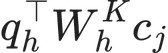
Whichever way you bracket it gives the same value (associativity), but a completely different algorithm:

On the left, expand the cached latent into a K first, then dot with the query. On the right, fold WK into the query first, then dot against the latent directly. The V side is the same idea in the other direction (section 3.2).
First difference: which side the projection lands on.
- expand: WKcj is done per cached token — once each, shared by every query token in the batch;
- absorb: (WK)⊤qh is done per query token — once each, shared across the whole history.
The widths involved:
- dc: the latent width, section 3’s cj — this is how wide each cached token is;
- dk: each head’s K after expanding;
- dv: each head’s V after expanding.
Second difference: how wide the remaining dot product is. For one query-token × cached-token pair, both paths do two multiply-accumulates — one to score, one to accumulate. The shapes make it clear.
After expanding:
- score: qh (1 × dk) dotted with kj,h (1 × dk), giving a scalar — dk MACs;
- weighted sum: the scalar ph,j times vj,h (1 × dv), accumulated into oh (1 × dv) — dv MACs.
Total dk + dv.
After absorbing:
- score: q̃h (1 × dc) dotted with cj (1 × dc) — dc MACs;
- weighted sum: the scalar ph,j times cj (1 × dc), accumulated into a dc-wide latent output — dc MACs.
Total 2dc.
The scoring difference is obvious (dk against dc). The accumulation is the one that is easy to miss: after expanding you accumulate a dv-wide v, while absorbing accumulates a dc-wide latent.
Worth stating plainly: both paths emit the same oh, both dv wide. That is exactly section 3.2’s step — multiplying by WV before the sum and after the sum are equal:
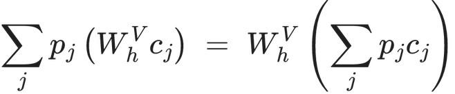
The only difference is which side of the sum WV is applied on. Expanding applies it first, once per cached token, so the accumulation is naturally dv wide. Absorbing applies it last, so the accumulation stays on the dc-wide latent and one final WV brings it back to dv — and that one runs once per query token, not once per pair.
It is the same fact as the K side above: bracketing changes the cost, not the answer.
Substituting Kimi K3 (dc = 512, dk = dv = 128): expanding gives 128 + 128 = 256, absorbing gives 2 × 512 = 1024.
For the same query/history pair, absorbing does 4× the arithmetic. The latent is wide, and dotting against it costs more — that intuition is correct.
The two paths in one sentence: expanding charges the projection to the history and gets a narrower dot product per pair; absorbing charges it to the query and pays for a wide latent on every pair.
5.2 One query token against one cached token
5.1 only counted the dot products. Each path also has its one projection, and adding it in is what shows who is cheaper at one-to-one.
Expanding: turning this cached token’s latent into K and V costs dc(dk + dv).
Absorbing: folding WK into the query and projecting the output back for this head also costs dc(dk + dv) — exactly the same.
For K3 (dc = 512, dk = dv = 128; DeepSeek-V3 has identical widths and only differs at 128 heads instead of 96), both projections come to 512 × 256 = 131072:
| projection | dot products | one-to-one total | |
|---|---|---|---|
| expand | 131072 | 256 | 131328 |
| absorb | 131072 | 1024 | 132096 |
So at one-to-one the outcome is decided entirely by the dot-product column — 5.1’s 4×. The projection column is identical and cancels.
At this point expanding looks like a free win.
5.3 Scaling up to S queries and L cached tokens
One-to-one cannot settle it, because in reality the two columns scale by different factors.
The dot-product column is straightforward: every query-token × cached-token pair pays it, so it scales with S·L.
The projection column is 5.1’s point — whichever side it lands on is the side whose count it is billed by:
- expand: WKcj is done per cached token, once each, shared by all query tokens in the batch → scales with L;
- absorb: (WK)⊤qh is done per query token, once each, shared across the whole history → scales with S.
One clarification: WK is per head, not shared across heads — in implementations the up-projection’s output dimension is H × (dk + dv) (in sglang, kv_b_proj is kv_lora_rank → num_heads * (qk_nope_head_dim + v_head_dim)). Expanding one cached token therefore has to be done once per head, with no sharing between heads.
But absorbing is per head too: (WK)⊤qh is also computed once per head. Both paths bill their projection per head, so H treats them equally — which is why arguing on a single head is not biased, and why H cancels out of the crossover later.
Multiplying through by H heads:
![F_{\text{MHA}} = 2H\left[\, L\,d_c(d_k+d_v) \;+\; S\,L\,(d_k+d_v) \,\right]](/zh/posts/attention-arithmetic-intensity/math/eq-82caa3df.jpg)
![F_{\text{MLA}} = 2H\left[\, S\,d_c(d_k+d_v) \;+\; S\,L\,\cdot 2d_c \,\right]](/zh/posts/attention-arithmetic-intensity/math/eq-aab5bbc3.jpg)
The difference is the first term: expanding multiplies by L, absorbing multiplies by S. Which is cheaper depends on whether S or L is larger in this forward pass — and decode and prefill sit at opposite ends of that question.
5.4 Decode: the MLA algorithm wins outright
In decode S = 1, one new token, and that projection has nothing to amortize against.
Substituting Kimi K3’s parameters into the two formulas above (96 heads, dc = 512, dk = dv = 128), per layer:
| L | MLA algorithm FLOPs / bytes / AI | MHA algorithm FLOPs / bytes / AI |
|---|---|---|
| 2,048 | 0.43 G / 2.10 M / 204 | 51.6 G / 103 M / 503 |
| 8,192 | 1.64 G / 8.39 M / 195 | 207 G / 411 M / 503 |
| 32,768 | 6.47 G / 33.6 M / 193 | 826 G / 1.64 G / 503 |
The MLA algorithm wins on both axes: 120× fewer FLOPs and 71× fewer bytes.
Nor is there room for “use the other one at short sequences”. Setting the two equal at S = 1 puts the crossing at L ≈ 1.006 — the MHA algorithm edges ahead only when the history contains a single token, and from L ≥ 2 onward the MLA algorithm wins throughout. The reason is plain: a longer L only scales that 120× gap up, it cannot reverse it.
5.5 Prefill: the other way around
Prefill computes a large batch of tokens at once, so S equals the sequence length, and the expansion is amortized across thousands of query tokens.
Same K3 parameters, same per layer:
| sequence length | MLA algorithm | MHA algorithm | MHA cheaper by |
|---|---|---|---|
| 2,048 | 464 G | 155 G | 3.00× |
| 8,192 | 6.80 T | 1.86 T | 3.67× |
| 32,768 | 106 T | 27.2 T | 3.91× |
There is no crossover in prefill — the MHA algorithm wins at every length. The reason is rather neat: when S = L, the per-token one-off cost is algebraically identical on both paths, 2HL·dc(dk+dv) — the MLA algorithm spends it folding WK into every query and projecting every output back, the MHA algorithm spends it expanding every cached token into K and V. They cancel, leaving only the ratio of the quadratic terms:
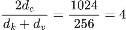
Longer sequences approach that 4×; shorter ones only shrink the advantage (3× at 2048) without reversing it.
5.6 So how large does S have to be?
The previous two sections each computed an extreme: decode at S = 1, where absorbing wins by 128×, and prefill at S in the thousands, where expanding wins by 4×. What about in between — how large does S have to get before you should switch?
The question has a definite answer. In 5.3’s two formulas the MLA one grows with S and the MHA one barely does, so there must be some S at which they tie; that S is the switch point, and solving FMLA = FMHA is how you find it.
First, what it looks like. With K3’s parameters and history length fixed at L = 32768, dividing one path’s FLOPs by the other — the x-axis is S, the y-axis is the ratio, and crossing 1 is where they tie:
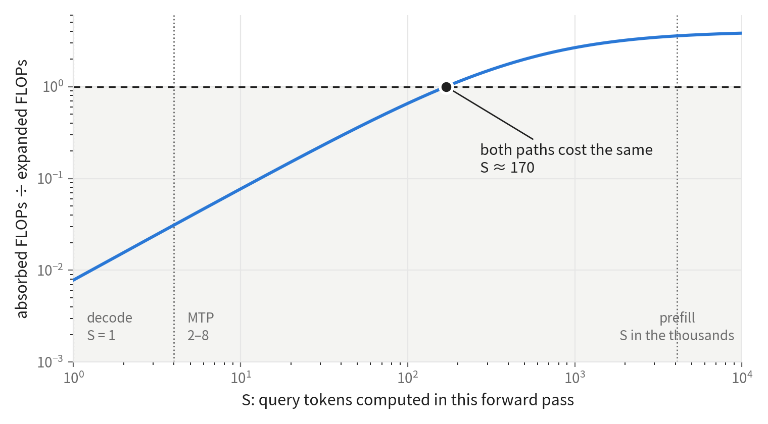
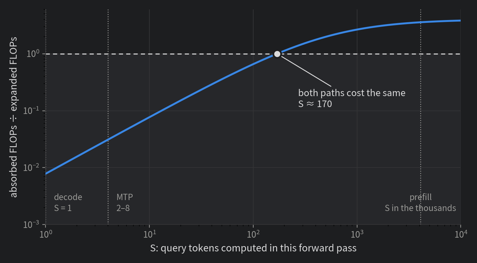
At the left end, decode’s ratio is only 0.008 — absorbing is more than 100× cheaper. The ratio climbs with S because both of the MLA path’s terms carry S, so every extra query token repeats the work, while the MHA path’s dominant term is the expansion, which carries only L — extra query tokens are nearly free. The curve crosses 1 at S ≈ 170.
Actually solving it shows H cancelling (both paths bill their projection per head, as 5.3 noted), leaving the crossing determined by a few head dims:

Substituting in, taking L from 512 up to 128K moves S* only from 128 to 171. In other words:
And because H cancels, DeepSeek-V3 (128 heads) and Kimi K3 (96 heads) have exactly the same crossover.
The three vertical lines say the rest: decode at S = 1 and MTP at 2–8 are pinned far to the left, while prefill, in the thousands, sits well to the right. Both regimes stay on their own side and almost nothing lands in between — so in practice this is never a “compute it and decide” question, but a straight dispatch on decode versus prefill.
5.7 Which is also where AI misleads
Section 1 left a thread hanging: AI only tells you which side of the roofline you are on. Here is the counterexample.
Look again at the decode rows in 5.4’s table: the MHA algorithm’s AI is 503, the MLA algorithm’s is 193. Read AI alone and you would pick the MHA algorithm — which in fact does 120× the FLOPs and touches 71× the bytes, both an order of magnitude or two worse. Its AI is higher precisely because the numerator exploded, not because it is a better deal.
Prefill fails differently: both paths land at AI in the 10⁵–10⁶ range, so AI only says “both deeply compute-bound” and cannot discriminate at all.
One gives the wrong answer, the other gives no answer. So:
AI is a ratio; it answers which side of the roofline you are on. To judge which path is faster, you have to put the absolute FLOPs and bytes side by side.
5.8 sglang dispatches exactly this way
This is not a paper exercise. The DeepSeek attention dispatch in sglang (python/sglang/srt/models/deepseek_common/attention_backend_handler.py) switches on forward mode:
- prefill goes to
MHA_ONE_SHOT/MHA_CHUNKED_KV, the expanding path; - decode, and speculative decoding’s verify / draft, go to
MLA, the absorbing path.
Notably, the decode path does not branch on L at all: the only place in the dispatch function that looks at sequence length is gated behind the prefill branch. That matches 5.4 — on the decode side there was never a window worth switching in.
6. Sparse attention reverses the direction
Section 5’s conclusion rests on one premise: attention looks at all L cached tokens. DeepSeek-V3.2’s DSA, and GLM’s equivalent, challenge exactly that premise — a lightweight selector scores the cached tokens and only the top-k actually participate. In V3.2’s config that k is index_topk = 2048.
This is not symmetric between the two algorithms:
- The MLA algorithm benefits from sparsity. The cache holds individual latents, so whichever 2048 are selected are gathered by index, and the scoring and weighted sum only run over those. The cost goes from L to k.
- The MHA algorithm does not. It has to expand the history into K and V and hand it to a dense GEMM — and the operators on that path only offer a dense GEMM, with no selective GEMM that runs on just the chosen tokens. So the expansion is still billed across the whole L.
The longer L gets, the more absurd the gap. With DeepSeek-V3’s parameters (128 heads), decode, per layer:
| L | MLA algorithm + sparse | MHA algorithm (dense) | gap |
|---|---|---|---|
| 2,048 | 0.57 G | 68.9 G | 121× |
| 8,192 | 0.57 G | 275 G | 483× |
| 32,768 | 0.57 G | 1.10 T | 1931× |
| 131,072 | 0.57 G | 4.41 T | 7725× |
The sparse path is flat past k; the dense one stays linear.
So once sparsity is in play, the direction of the choice flips relative to section 5: dense says “the longer the sequence, the more you want the MHA algorithm”, sparse says “the longer the sequence, the more you want the MLA algorithm”. sglang’s DSA dispatch (dsa_backend.py) confirms it — the MHA algorithm is used only when max_kv_len is under a threshold, above which it uses sparse MLA, and decode / verify always go to MLA.
That threshold defaults to 2048 — exactly index_topk. The meaning is clear: below 2048 the top-k selects everything, sparsity buys nothing, and the faster dense kernel is preferable; above it, sparsity finally starts saving something real.
7. The four structures side by side
Everything below is BF16, single-token decode, counting only the attention core’s one pass over the cached KV, assuming a fused kernel and ignoring softmax / projections / output projection as lower-order terms.
| Attention | cache structure | main reuse | BF16 decode AI |
|---|---|---|---|
| MHA | each query head has its own K/V | essentially no cross-head reuse | 1 |
| GQA | a group of query heads shares K/V | KV reused across query heads | Hq/Hkv |
| MQA | all query heads share one K and one V | maximal cross-head reuse | Hq |
| MLA | one latent | cross-head reuse + one latent serving as both K and V | 2Hq |
| DeepSeek V3/R1 | one latent, 128 heads | as above | 256 FLOP/B |
| Kimi K3’s MLA layer | one latent, 96 heads | as above | 192 FLOP/B |
Compressed into a single line:
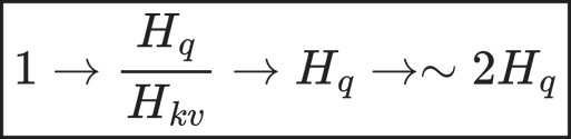
I find this view more unifying than “how much KV cache does variant X save”:
A large part of how attention architectures have evolved is the design of data reuse. GQA and MQA reuse KV across query heads; MLA goes further and has one latent serve as both K and V.
8. Why MLA and MTP fight each other
Now the opening quote can be revisited.
Ordinary autoregressive decode has one query token per step. The systems intuition behind MTP and speculative decoding is: since the KV cache has already been dragged in from HBM, can it serve several candidate tokens at once?
Say one verification step uses the same cached history to serve S query positions. To a very rough approximation the HBM traffic does not grow proportionally with S while the QK/PV computation scales nearly linearly with it, so:

For plain MQA:

and for MLA:
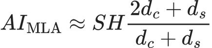
This also answers a question in passing: MTP lifts the query token count from 1 to S, so does it push past section 5’s crossover and switch to the MHA algorithm? No. Speculation windows are typically 2 to 8, at most a few dozen, nowhere near 171. So MTP stays on the MLA-algorithm side — every query token still runs against the wide latent. Which is exactly why its AI climbs faithfully with S.
In other words, MTP and MLA are spending the same resource: the GPU compute left idle by a memory-bound decode.
- MLA spends extra compute to buy stronger cache reuse;
- MTP spends extra speculative / verification compute to buy fewer serial decoding steps.
If the workload were a low-AI MQA, say AI ≈ 70–100, the GPU is far from the roofline knee and MTP’s extra arithmetic is largely using tensor cores that were idle anyway.
But DeepSeek-style MLA already reaches, at a single query:

and Kimi K3’s MLA layer:

Against the theoretical balance points above — H200 at ~206 FLOP/B, H100 and B200 in the two-to-three-hundred range.
So at S = 1 MLA has already moved decode from clearly memory-bound to roughly the compute/memory balance point. Take S to 2:


and it sails past the roofline knee into compute-bound territory.
At that point MTP’s extra arithmetic is no longer using otherwise idle compute; it starts costing real latency.
So the opening claim — that MLA behaves during decoding like an MQA with head_dims=512+ and has already consumed most of the compute — reduces, as I now understand it, to:
MLA and MTP are both making a compute-for-bandwidth / compute-for-latency trade. MLA has already spent a large part of decode’s idle compute headroom, leaving less of it free for MTP.
Mathematically, MLA’s AI is “only” a constant factor under 2 above MQA’s. Systems-wise, that constant is exactly enough to push the workload across the roofline.
Which is the part I find most interesting.
Acknowledgements
Thanks to Yangmin for the insights and discussion on MLA inference.
After finishing this I found that Zyphra’s Compressed Convolutional Attention (arXiv:2510.04476) states the same thing independently, in nearly the same terms:
MLA has an arithmetic intensity of 2n_heads at inference time, which is very large, and targets the ridge of the roofline plot on a H100 for a single query. … The arithmetic intensity required to breach the ridge of the roofline for an Nvidia H100 under bfloat16 is 295 FLOPs per byte. Deepseek seemingly chose their number of heads for the DeepseekV3 model to accordingly saturate the roofline to approach compute bound inference at batch size 1. … This falls short in cases where speculative decoding is utilized such that the arithmetic intensity passes the roofline.
AI = 2H, 295 FLOP/B, and “DeepSeek picked their head count against the roofline” — all three line up. It also raises an angle this post does not cover: MLA also loses under tensor parallelism, because the shared KV has to be replicated per TP rank, which gives back the reuse MQA had bought.
One more line from that paper, which closes section 5’s observation about AI nicely:
while MLA is capable of better compute utilization on decode, the increase in FLOPs that would otherwise go unused does not automatically result in victory. Model quality and latency, not SM utilization, is the end goal.
Appendix A: putting RoPE back
The AI = 2H above is the cleanest form of the result, but it rests on ignoring RoPE. Here it comes back.
The problem is at 3.1’s absorption step, which relies on associativity to move WK over to the query side. RoPE is a position-dependent rotation sitting between query and key, and the two sides are rotated by different angles, so that regrouping no longer works — with RoPE in place you cannot score against the latent directly.
DeepSeek’s answer is a division of labor: the latent part is absorbed as usual and carries no RoPE, while a separate small segment of RoPE-carrying key is kept, shared by all heads and stored in the cache alongside the latent. That segment only participates in scoring, not in the final weighted sum (it has no corresponding Value).
Writing its width as:

each cached token’s real width is:
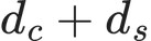
the QK contraction width is:
and the PV contraction width is still only:

so:

that is:

HBM traffic:
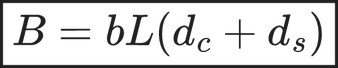
giving:
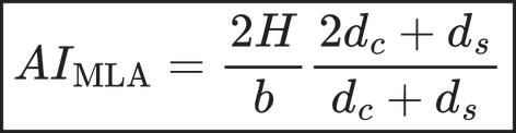
and with BF16:
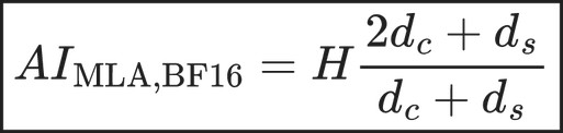
When ds ≪ dc the factor naturally approaches:

A.1 DeepSeek V3 / R1
From the DeepSeek-V3 config:

so:


A.2 Kimi K3
From the Kimi K3 config’s MLA layer:

so:
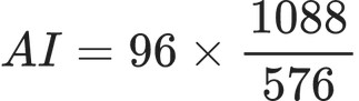

K3 has an implementation quirk: the config keeps the qk_rope_head_dim=64 layout but also sets mla_use_nope=true, so those 64 dims are not actually doing RoPE. That does not affect the derivation here — all we need is that it is likewise a small segment shared by all heads, participating only in scoring and not in the weighted sum, 64 wide, substituted into the formulas above.
A.3 Section 5’s numbers
Section 5’s comparison of the two algorithms used the same simplification. Adding the segment back:
| main text (simplified) | with the segment | |
|---|---|---|
| per pair, absorb | 1024 | 1088 |
| per pair, expanded | 256 | 320 |
| expansion, per cached token | 131072 | 131072 |
| per-pair ratio | 4.0× | 3.4× |
The expansion is unchanged, because the segment is shared across heads and does not need expanding per head. Both per-pair costs widen, so the ratio drops from 4 to 3.4, and the MHA algorithm’s prefill advantage drops from about 3.9× to about 3.3×.
The crossover does not move at all: it is the expansion divided by the per-pair difference, and that difference is 1024 − 256 = 768 before and 1088 − 320 = 768 after — identical. So S* ≈ 171 is unaffected.